The moment-generating function of the gamma distribution is \( M(t) = (1-\theta t)^{-\alpha}\). Such a friendly little guy. Not what you would expect when you start with this:

$$ M(t) = \int_{0}^{\infty}e^{tx}\frac{1}{\Gamma (\alpha)\theta^{\alpha}}x^{\alpha – 1}e^{-x/\theta}dx$$

How do we get there? First let’s combine the two exponential terms and move the gamma fraction out of the integral:

$$ M(t) = \frac{1}{\Gamma (\alpha)\theta^{\alpha}}\int_{0}^{\infty}x^{\alpha – 1}e^{tx-x/\theta}dx$$

Multiply \( tx\) in the exponential by \( \frac{\theta}{\theta} = 1\), add the two terms together and factor out \( -x\):

$$ M(t) = \frac{1}{\Gamma (\alpha)\theta^{\alpha}}\int_{0}^{\infty}x^{\alpha – 1}e^{-x(1-\theta t)/\theta}dx$$

Now we’re ready to do so substitution in the integral. Let \( u = \frac{x(1-\theta t)}{\theta}\). That means we have \( du = \frac{1-\theta t}{\theta}dx\). Now solve those for x and dx, respectively. We get \( x = \frac{\theta u}{1-\theta t}\) and \( dx = \frac{\theta}{1-\theta t}du\). Now substitute those in the integral to see something that looks truly awful:

$$ M(t) = \frac{1}{\Gamma (\alpha)\theta^{\alpha}}\int_{0}^{\infty}\frac{\theta u}{1-\theta t}^{\alpha – 1}e^{-u}\frac{\theta}{1-\theta t}du$$

If re-write everything inside the integral with exponents we can do some cancellation and make this integral more attractive:

$$ M(t) = \frac{1}{\Gamma (\alpha)\theta^{\alpha}}\int_{0}^{\infty}(1-\theta t)^{-\alpha + 1}(1-\theta t)^{-1}(\theta u)^{\alpha-1}\theta e^{-u}du$$

Using the rules of exponents we see that \( (1-\theta t)^{-\alpha + 1}(1-\theta t)^{-1} = (1- \theta t)^{-\alpha}\) which can be moved out of the integral since it doesn’t have \( u\) in it:

$$ M(t) = \frac{(1- \theta t)^{-\alpha}}{\Gamma (\alpha)\theta^{\alpha}}\int_{0}^{\infty}(\theta u)^{\alpha-1}\theta e^{-u}du$$

Using the rules of exponents again we see that \( \theta^{\alpha -1}\theta = \theta^{\alpha}\):

$$ M(t) = \frac{(1- \theta t)^{-\alpha}}{\Gamma (\alpha)\theta^{\alpha}}\int_{0}^{\infty}\theta^{\alpha}u^{\alpha – 1} e^{-u}du$$

Now notice we can cancel out the two \( \theta^{\alpha}\) terms:

$$ M(t) = \frac{(1- \theta t)^{-\alpha}}{\Gamma (\alpha)}\int_{0}^{\infty}u^{\alpha – 1} e^{-u}du$$

The integral is now the gamma function: \( \Gamma (\alpha) = \int_{0}^{\infty}u^{\alpha – 1} e^{-u}du\). Make that substitution:

$$ M(t) = \frac{(1- \theta t)^{-\alpha}}{\Gamma (\alpha)}\Gamma(\alpha)$$

Cancel out the \( \Gamma(\alpha)\) terms and we have our nice-looking moment-generating function:

$$ M(t) = (1- \theta t)^{-\alpha}$$

If we take the derivative of this function and evaluate at 0 we get the mean of the gamma distribution:

$$ M'(t) = -\alpha (1-\theta t)^{-\alpha -1}(-\theta)$$

$$ M'(0) = -\alpha(1 – 0)^{-\alpha -1}(-\theta) = \alpha\theta = E(X)$$

Recall that \( \theta\) is the mean time between events and \( \alpha\) is the number of events. Multiply them together and you have the mean. This makes sense. If the mean wait time between events is 2 minutes (\( \theta = 2\)) and we’re interested in the distribution of times until 4 events occur (\( \alpha = 4\)), it seems reasonable to think the mean wait time to observe the 4th event would be 8 minutes (\( 4(2)\)).

If we take the second derivative of the moment-generating function and evaluate at 0, we get the second moment about the origin which we can use to find the variance:

$$ M”(t) = (-\alpha – 1)\theta\alpha(1-\theta t)^{-\alpha – 2}(-\theta)$$

$$ M”(0) = (-\alpha – 1)\theta\alpha(1-0)^{-\alpha – 2}(-\theta) = (-\alpha – 1)(-\theta^{2})\alpha$$

Now find the variance:

$$ Var(X) = (-\alpha – 1)(-\theta^{2})\alpha – (\alpha\theta)^{2}$$

$$ Var(X) = \alpha^{2}\theta^{2} + \alpha\theta^{2} – \alpha^{2}\theta^{2}$$

$$ Var(X) = \alpha\theta^{2}$$

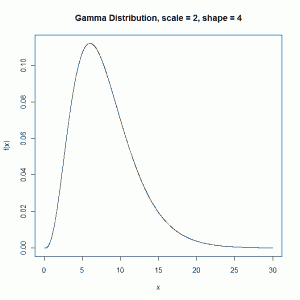
Going back to our example with \( \alpha = 4\) (number of events) and \( \theta=2\) (mean time between events), we have as our variance \( 4(2^{2})=16\). The square root of that gives our standard deviation as 4.

Plugging the mean and standard deviation into the dgamma function in R, we can plot this particular gamma distribution:

xval <- seq(0,30, by = 0.01)
ga.4 <- dgamma(xval, shape=4, scale=2)
plot(xval,ga.4,col=1, type = "l", ylab="f(x)", xlab="x")
title(main="Gamma Distribution, scale = 2, shape = 4")