library(rstanarm)
data <- read.table("https://github.com/avehtari/ROS-Examples/raw/refs/heads/master/NES/data/nes.txt")In section 10.9 of Regression and Other Stories, the authors introduce the idea of fitting the same model to many data sets. They begin the section by saying, “it is common to fit a regression model repeatedly…to subsets of an existing data set.” But then two paragraphs later call this idea a “secret weapon” because “it is so easy and powerful but yet is rarely used.” So which is it? Common or rarely used?
Anyway, here’s the code they use to demonstrate this idea using NES data. This creates Figure 10.9 on page 149. While I enjoyed working through this code and figuring out how it works, I decided to re-implement it using data frames and ggplot2.
First I load the {rstanarm} package and read in the data.
Next I modify their custom function as follows. The changes are in the coefs object that is created. Instead of a vector, I return a data frame. I also add the variable name and year to the data frame.
coef_names <- c("Intercept", "Ideology", "Black", "Age_30_44",
                "Age_45_64", "Age_65_up", "Education", "Female", "Income")
regress_year <- function (yr) {
  this_year <- data[data$year==yr,]
  fit <- stan_glm(partyid7 ~ real_ideo + race_adj + factor(age_discrete) +
                    educ1 + female + income,
                  data=this_year, warmup = 500, iter = 1500, refresh = 0,
                  save_warmup = FALSE, cores = 1, open_progress = FALSE)
    coefs <- data.frame(var = coef_names,
                      coef = coef(fit),
                      se = se(fit),
                      year = yr)
}
Now I run the function using lapply(), combine the list of data frames into one data frame, add upper and lower limits of a 50% confidence interval, and set the variable name as a factor.
sum2 <- lapply(seq(1972,2000,4), regress_year)
sumd <- do.call(rbind, sum2)
sumd$upper <- sumd$coef + sumd$se*0.67
sumd$lower <- sumd$coef - sumd$se*0.67
sumd$var <- factor(sumd$var, levels = coef_names)
And finally I create the plot using {ggplot2}.
library(ggplot2)
ggplot(sumd) +
  aes(x = year, y = coef) +
  geom_point() +
  geom_errorbar(mapping = aes(ymin = lower, ymax = upper), width = 0) +
  geom_hline(yintercept = 0, linetype = 2) +
  facet_wrap(~ var, scales = "free") +
  theme_classic()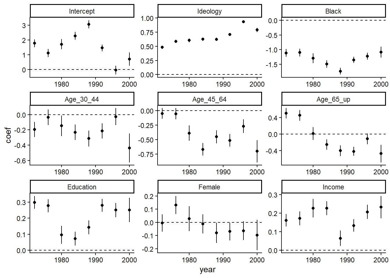
According to the book, “ideology and ethnicity are the most important, and their coefficients have been changing over time.”
The above approach uses Bayesian modeling via the {rstanarm} package. We can also deploy the secret weapon using a frequentist approach via the lmList() function from the {lme4} package. Below I first subset the data to select only the columns I need for the years 1972 - 2000. This is necessary due to the amount of missingness in the data.
library(lme4)
vars <- c("partyid7", "real_ideo" , "race_adj" , "age_discrete" ,
  "educ1" , "female" , "income", "year")
d <- data[data$year %in% seq(1972,2000,4),vars]
fm1 <- lmList(partyid7 ~ real_ideo + race_adj + factor(age_discrete) +
                educ1 + female + income | year,
              data = d)
Calling summary on the object lists a summary of coefficients over time.
summary(fm1)Call:
Model: partyid7 ~ real_ideo + race_adj + factor(age_discrete) + educ1 + female + income | NULL
Data: d
Coefficients:
(Intercept)
Estimate Std. Error t value Pr(>|t|)
1972 1.76583047 0.3713743 4.7548538 2.019151e-06
1976 1.11162271 0.4038796 2.7523615 5.929490e-03
1980 1.70511202 0.5101462 3.3423987 8.342261e-04
1984 2.27900236 0.3731396 6.1076403 1.056356e-09
1988 3.04892311 0.4003568 7.6155146 2.913307e-14
1992 1.44675559 0.3479402 4.1580579 3.241743e-05
1996 -0.06088684 0.4523491 -0.1346014 8.929303e-01
2000 0.71444233 0.6875610 1.0390967 2.987898e-01
real_ideo
Estimate Std. Error t value Pr(>|t|)
1972 0.4846373 0.04058343 11.94175 1.320025e-32
1976 0.5874170 0.04129972 14.22327 2.220613e-45
1980 0.6039183 0.04995714 12.08873 2.298924e-33
1984 0.6262146 0.03860522 16.22098 2.771748e-58
1988 0.6219214 0.03971156 15.66097 1.659414e-54
1992 0.7075364 0.03500057 20.21499 9.375655e-89
1996 0.9364460 0.04067273 23.02393 8.874569e-114
2000 0.7892252 0.06129477 12.87590 1.399443e-37
race_adj
Estimate Std. Error t value Pr(>|t|)
1972 -1.105586 0.1870994 -5.909083 3.575067e-09
1976 -1.097028 0.1980980 -5.537805 3.155805e-08
1980 -1.284468 0.2429898 -5.286098 1.281122e-07
1984 -1.483666 0.1812912 -8.183885 3.153604e-16
1988 -1.732068 0.1721402 -10.061961 1.109738e-23
1992 -1.346218 0.1564942 -8.602349 9.232858e-18
1996 -1.220354 0.1846709 -6.608263 4.126844e-11
2000 -1.079103 0.2948775 -3.659496 2.542700e-04
factor(age_discrete)2
Estimate Std. Error t value Pr(>|t|)
1972 -0.18895861 0.1373869 -1.3753757 0.16905188
1976 -0.03744826 0.1486541 -0.2519154 0.80111262
1980 -0.14625870 0.1939140 -0.7542451 0.45072333
1984 -0.23055707 0.1410016 -1.6351374 0.10205793
1988 -0.30995572 0.1512620 -2.0491320 0.04048039
1992 -0.21210428 0.1482977 -1.4302602 0.15267977
1996 -0.02979256 0.1829521 -0.1628435 0.87064561
2000 -0.45006072 0.2959671 -1.5206443 0.12838698
factor(age_discrete)3
Estimate Std. Error t value Pr(>|t|)
1972 -0.04740623 0.1347712 -0.3517535 7.250320e-01
1976 -0.05728971 0.1461493 -0.3919945 6.950723e-01
1980 -0.38373449 0.1947510 -1.9703849 4.882726e-02
1984 -0.66715561 0.1531480 -4.3562810 1.338718e-05
1988 -0.45235822 0.1629587 -2.7759065 5.517059e-03
1992 -0.50779145 0.1591265 -3.1911175 1.422483e-03
1996 -0.27181837 0.1907075 -1.4253153 1.541034e-01
2000 -0.71662580 0.2995257 -2.3925355 1.675438e-02
factor(age_discrete)4
Estimate Std. Error t value Pr(>|t|)
1972 0.5125853 0.1772718 2.8915225 0.003843694
1976 0.4486697 0.1889933 2.3739982 0.017619118
1980 0.0238989 0.2292029 0.1042696 0.916957892
1984 -0.2458586 0.1823842 -1.3480260 0.177686577
1988 -0.4002949 0.1916484 -2.0886944 0.036765446
1992 -0.4130676 0.1714062 -2.4098761 0.015979426
1996 -0.1150134 0.2071408 -0.5552427 0.578743539
2000 -0.4803803 0.3324209 -1.4450965 0.148468300
educ1
Estimate Std. Error t value Pr(>|t|)
1972 0.29708140 0.05826098 5.099149 3.486782e-07
1976 0.27725165 0.06059524 4.575469 4.820110e-06
1980 0.09550340 0.08261012 1.156074 2.476841e-01
1984 0.07262794 0.06501416 1.117110 2.639796e-01
1988 0.14341231 0.06473108 2.215509 2.675200e-02
1992 0.28034637 0.05916944 4.738026 2.193737e-06
1996 0.25114897 0.07093933 3.540335 4.017956e-04
2000 0.24461379 0.10801197 2.264692 2.355714e-02
female
Estimate Std. Error t value Pr(>|t|)
1972 -0.005967246 0.10018983 -0.0595594 0.9525080
1976 0.133917095 0.10627385 1.2601133 0.2076637
1980 0.028503792 0.13923027 0.2047241 0.8377927
1984 -0.013415054 0.10477430 -0.1280376 0.8981223
1988 -0.079195190 0.11057733 -0.7161974 0.4738895
1992 -0.068672465 0.09994152 -0.6871265 0.4920221
1996 -0.059622697 0.11476049 -0.5195403 0.6033978
2000 -0.094042287 0.17291800 -0.5438548 0.5865559
income
Estimate Std. Error t value Pr(>|t|)
1972 0.16082722 0.05077800 3.167262 1.544359e-03
1976 0.17180218 0.05780102 2.972303 2.964176e-03
1980 0.22816242 0.07197937 3.169831 1.530785e-03
1984 0.22486650 0.05569547 4.037429 5.452323e-05
1988 0.06352031 0.05891789 1.078116 2.810132e-01
1992 0.13290845 0.05188253 2.561719 1.043296e-02
1996 0.20801839 0.05996115 3.469220 5.246072e-04
2000 0.23581142 0.08847826 2.665190 7.709274e-03
Residual standard error: 1.815982 on 8351 degrees of freedomTo create the plot, I need to do some data wrangling. Below I extract the coefficients from the summary, which returns an array. I then use the adply() function from the {plyr} package to convert the array to a data frame. Then I add year, upper 50% CI limit, and lower 50% CI limit to the data frame. I also change the variable column to a factor so the order of the coefficients will be preserved in the plot.
sout <- summary(fm1)$coefficients

library(plyr)
sumd2 <- adply(sout, .margins = 3, .id = "Var")
sumd2$year <- seq(1972,2000,4)
sumd2$upper <- sumd2$Estimate + sumd2$`Std. Error`*0.67
sumd2$lower <- sumd2$Estimate - sumd2$`Std. Error`*0.67
sumd2$Var <- factor(sumd2$Var, labels = coef_names)
And once again I create the plot.
ggplot(sumd2) +
  aes(x = year, y = Estimate) +
  geom_point() +
  geom_errorbar(mapping = aes(ymin = lower, ymax = upper), width = 0) +
  geom_hline(yintercept = 0, linetype = 2) +
  facet_wrap(~ Var, scales = "free") +
  theme_classic()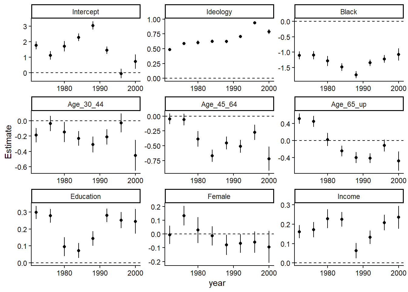
The result is almost identical to the one created using {rstanarm}.