For a few years now I’ve been chipping away at Regression Modeling Strategies by Frank Harrell. Between the exposition, the case studies, the notes, the references, the code and exercises, it’s a deep and rich source of statistical learning. The book’s associated R package, {rms}, is used throughout the book and is one of the reasons it can be tough sledding at times, especially if you’re like me and learned regression using the base R functions lm() and glm(). In this post I want to create a Rosetta stone of sorts that shows how to replicate what {rms} does using base R and other packages. Hopefully this will help a few random internet strangers get a better grip on {rms}.
Model fitting and summary output
To begin, let’s load the gala data from the {faraway} package. The gala data set contains data on species diversity on the Galapagos Islands. Below we use the base R lm() function to model the number of plant Species found on the island as function of the Area of the island (km\(^2\)), the highest Elevation of the island (m), the distance from the Nearest island (km), the distance from Santa Cruz island (km), and the area of the Adjacent island (square km). This how I and thousands of others learned to do regression in R. Of course we use the familiar summary() function on our model object to see the model coefficients, marginal tests, the residual standard error, R squared, etc.
library(faraway)data("gala")m <-lm(Species ~ Area + Elevation + Nearest + Scruz + Adjacent, data = gala)summary(m)
Call:
lm(formula = Species ~ Area + Elevation + Nearest + Scruz + Adjacent,
    data = gala)

Residuals:
     Min       1Q   Median       3Q      Max
-111.679  -34.898   -7.862   33.460  182.584

Coefficients:
             Estimate Std. Error t value Pr(>|t|)
(Intercept)  7.068221  19.154198   0.369 0.715351
Area        -0.023938   0.022422  -1.068 0.296318
Elevation    0.319465   0.053663   5.953 3.82e-06 ***
Nearest      0.009144   1.054136   0.009 0.993151
Scruz       -0.240524   0.215402  -1.117 0.275208
Adjacent    -0.074805   0.017700  -4.226 0.000297 ***
---
Signif. codes:  0 '***' 0.001 '**' 0.01 '*' 0.05 '.' 0.1 ' ' 1

Residual standard error: 60.98 on 24 degrees of freedom
Multiple R-squared:  0.7658,    Adjusted R-squared:  0.7171
F-statistic:  15.7 on 5 and 24 DF,  p-value: 6.838e-07
Now let’s fit the same model using the {rms} package. For this we use the ols() function. Notice we can use R’s formula syntax as usual. One additional argument we need to use that will come in handy in a few moments is x = TRUE. This stores the predictor variables with the model fit as a design matrix. Notice we don’t need to call summary() on the saved model object. We simply print it.
library(rms)mr <-ols(Species ~ Area + Elevation + Nearest + Scruz + Adjacent, data = gala, x =TRUE)mr
Linear Regression Model

ols(formula = Species ~ Area + Elevation + Nearest + Scruz +
    Adjacent, data = gala, x = TRUE)

                 Model Likelihood    Discrimination
                       Ratio Test           Indexes
Obs       30    LR chi2     43.55    R2       0.766
sigma60.9752    d.f.            5    R2 adj   0.717
d.f.      24    Pr(> chi2) 0.0000    g      105.768

Residuals

     Min       1Q   Median       3Q      Max
-111.679  -34.898   -7.862   33.460  182.584

          Coef    S.E.    t     Pr(>|t|)
Intercept  7.0682 19.1542  0.37 0.7154
Area      -0.0239  0.0224 -1.07 0.2963
Elevation  0.3195  0.0537  5.95 <0.0001
Nearest    0.0091  1.0541  0.01 0.9932
Scruz     -0.2405  0.2154 -1.12 0.2752
Adjacent  -0.0748  0.0177 -4.23 0.0003
The coefficient tables and summaries of residuals are the same. Likewise both return R-squared and Adjusted R-squared. The residual standard error from the lm() output is called sigma in the ols() output.
The ols output also includes a “g” statistic. This is Gini’s mean difference and measures the dispersion of predicted values. It’s an alternative to standard deviation. We can use the {Hmisc} function GiniMd to calculate Gini’s mean difference for the model fit with lm() as follows.
Hmisc::GiniMd(predict(m))
[1] 105.7677
Whereas the summary output for lm() includes an F test for the null that all of the predictor coefficients equal 0, the ols() function reports a Likelihood Ratio Test. This tests the same null hypothesis using a ratio of likelihoods. We can calculate this test for the lm() model using the logLik() function. First we subtract the log likelihood of a model with no predictors from the log likelihood for the original model, and then multiply by 2. Apparently, according to Wikipedia, multiplying by 2 ensures mathematically that the test statistic converges to a chi-square distribution if the null is true. If the null is true, we expect this different of log likelihoods (or ratio, according to the quotient rule of logs) to be about 1. This statistic is very large. Clearly at least one of the predictor coefficients is not 0.
If we wanted to calculate the p-value that appears in the ols() output, we can use the pchisq() function. Obviously the p-value in the ols() output is rounded.
pchisq(LRchi2, df =7, lower.tail =FALSE)
'log Lik.' 2.60758e-07 (df=7)
Partial F tests and important measures
Now let’s use the anova() function on both model objects and compare the output. For the lm() object, we get sequential partial F tests using Type I sums of squares. Each line tests the null hypothesis that adding the listed predictor to the previous model without it explains no additional variability. So the Area line compares a model with just an intercept to a model with an intercept and Area. The Elevation line compares a model with an intercept and Area to a model with an intercept, Area, and Elevation. And so on. Small p-values are evidence against the null.
anova(m)
Analysis of Variance Table

Response: Species
          Df Sum Sq Mean Sq F value    Pr(>F)
Area       1 145470  145470 39.1262 1.826e-06 ***
Elevation  1  65664   65664 17.6613 0.0003155 ***
Nearest    1     29      29  0.0079 0.9300674
Scruz      1  14280   14280  3.8408 0.0617324 .
Adjacent   1  66406   66406 17.8609 0.0002971 ***
Residuals 24  89231    3718
---
Signif. codes:  0 '***' 0.001 '**' 0.01 '*' 0.05 '.' 0.1 ' ' 1
Calling anova() on the ols() object produces a series of partial F tests using Type II sums of squares. Each line tests the null hypothesis that adding the listed predictor to a model with all the other listed predictors already in it explains no additional variability. So the Area line compares a model with all the other predictors to a model with all the other predictors and Area. The Elevation line compares a model with all the other predictors to a model with all the other predictors and Elevation. The final line labeled REGRESSION is the F Test reported in the summary output for the lm() model.
anova(mr)
                Analysis of Variance          Response: Species

 Factor     d.f. Partial SS   MS           F     P
 Area        1   4.237718e+03 4.237718e+03  1.14 0.2963
 Elevation   1   1.317666e+05 1.317666e+05 35.44 <.0001
 Nearest     1   2.797576e-01 2.797576e-01  0.00 0.9932
 Scruz       1   4.635787e+03 4.635787e+03  1.25 0.2752
 Adjacent    1   6.640639e+04 6.640639e+04 17.86 0.0003
 REGRESSION  5   2.918500e+05 5.837000e+04 15.70 <.0001
 ERROR      24   8.923137e+04 3.717974e+03
To run these same Partial F tests for the lm() object we can use the base R drop1() function.
drop1(m, test ="F")
Single term deletions

Model:
Species ~ Area + Elevation + Nearest + Scruz + Adjacent
          Df Sum of Sq    RSS    AIC F value    Pr(>F)
<none>                  89231 251.93
Area       1      4238  93469 251.33  1.1398 0.2963180
Elevation  1    131767 220998 277.14 35.4404 3.823e-06 ***
Nearest    1         0  89232 249.93  0.0001 0.9931506
Scruz      1      4636  93867 251.45  1.2469 0.2752082
Adjacent   1     66406 155638 266.62 17.8609 0.0002971 ***
---
Signif. codes:  0 '***' 0.001 '**' 0.01 '*' 0.05 '.' 0.1 ' ' 1
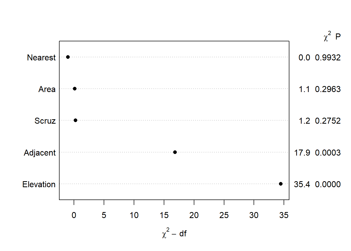
The {rms} package offers a convenient plot method for anova() objects that “draws dot charts depicting the importance of variables in the model” (from the anova.rms help page). The default importance measure is the chi-square statistic for each factor minus its degrees of freedom. There are several other importance measures available. See the anova.rms help page for the what argument.
plot(anova(mr))
IQR effect plots
Earlier we noted that we don’t use the summary() function on ols() model objects to see a model summary. That doesn’t mean there isn’t a summary() method available. There is, but it does something entirely different than the summary method for lm() objects. If we try it right now we get an error message:
summary(mr)
Error in summary.rms(mr): adjustment values not defined here or with datadist for Area Elevation Nearest Scruz Adjacent
Notice what it says: “adjustment values not defined here or with datadist”. This tells us we need to define “adjustment values” to use the summary() function. Instead of summarizing the model, the {rms} summary function when called on {rms} model objects returns a “summary of the effects of each factor”. Let’s demonstrate what this means.
The easiest way to define adjustment values is to use the datadist() function on our data frame and then set the global datadist option using the base R options() function. Harrell frequently assigns datadist results to “d” so we do the same. (Also, the help page for datadist states, “The best method is probably to run datadist once before any models are fitted, storing the distribution summaries for all potential variables.” I elected to wait for presentation purposes.)
d <-datadist(gala)options(datadist ="d")
If we print “d” we see adjustment levels for all variables in the model.
This produces an interquartile range “Effects” summary for all predictors. For example, in the first row we see the effect of Area is about -1.41. To calculate this we predict Species when Area = 59.238 (High, 75th percentile) and when Area = 0.2575 (Low, 25th percentile) and take the difference in predicted species. For each prediction, all other variables are held at their “Adjust to” level as shown above when we printed the datadist object. In addition to the effect, the standard error (SE) of the effect and a 95% confidence interval on the effect is returned. In this case we’re not sure if the effect is positive or negative. (Incidentally )
To calculate this effect measure using our lm() model object we can use the predict() function to make two predictions and then take the difference using the diff() function. Notice all the values in the newdata argument come from the datadist object above. The two values for Area are the “Low:effect” and “High:effect” values. The other values from the “Adjust to” row.
# How to get Area effect in summary(mr) output = -1.411900p <-predict(m, newdata =data.frame(Area =c(0.2575, 59.238), Elevation=97.75, Nearest=3.05,Scruz=46.65,Adjacent=2.59))p
       1        2
26.90343 25.49153
diff(p)
        2
-1.411895
To get the standard error and confidence interval we can do the following. (Recall 58.980 is the IQR of Area.)
se <-sqrt((58.980*vcov(m)["Area","Area"] *58.980))se
[1] 1.32247
diff(p) +c(-1,1) * se *qt(0.975, df =24)
[1] -4.141340 1.317549
This is made a little easier using the emmeans() function in the {emmeans} package. We use the at argument to specify at what values we wish to make predictions for Area. All other values are held at their median by setting cov.reduce = median. Sending the result to the {emmeans} function contrast with argument “revpairwise” says to subtract the estimated means in reverse order. Finally we pipe into the confint() to replicate the IQR effect estimate for Area that we saw in the ols() summary.
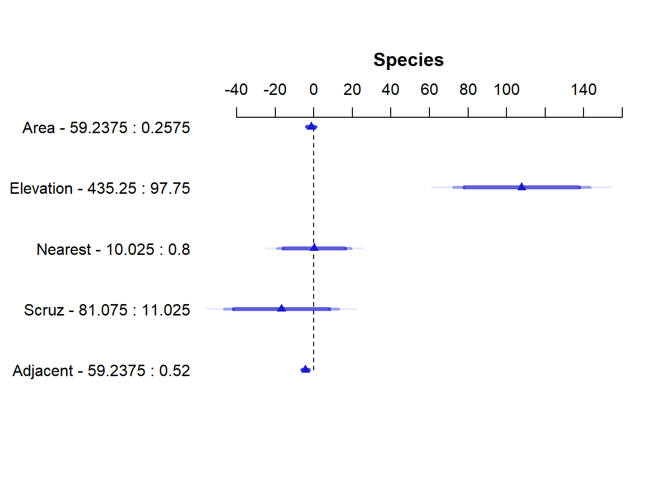
There is also a plot method for {rms} summary objects. It plots the Effects and the 90, 95, and 99 percent confidence intervals using different shades of blue. Below we see the Area effect of -1.41 with relatively tight confidence intervals hovering around 0.
plot(summary(mr))
Non-linear effects
Harrell advocates using non-linear effects in the form of regression splines. This makes a lot of sense when you pause and consider how many effects in real life are truly linear. Not many. Very few associations in nature indefinitely follow a straight line relationship. Fortunately, we can easily implement regression splines in R and specify how much non-linearity we want to entertain. We do this either in the form of degrees of freedom or knots. More of both means more non-linearity. I personally think of it as the number of times the relationship might change direction.
One way to implement regression splines in R is via the ns() function in the {splines} package, which comes installed with R. Below we fit a model that allows the effect of Nearest to change directions three times by specifying df=3. We might think of this as sort of like using a 3-degree polynomial to model Nearest (but that’s not what we’re doing). The summary shows three coefficients for Nearest, neither of which have any interpretation.
library(splines)m2 <-lm(Species ~ Area + Elevation +ns(Nearest, df =3) + Scruz + Adjacent, data = gala)summary(m2)
Call:
lm(formula = Species ~ Area + Elevation + ns(Nearest, df = 3) +
    Scruz + Adjacent, data = gala)

Residuals:
    Min      1Q  Median      3Q     Max
-79.857 -28.285  -0.775  25.498 163.069

Coefficients:
                       Estimate Std. Error t value Pr(>|t|)
(Intercept)            13.18825   27.39386   0.481   0.6350
Area                   -0.03871    0.02098  -1.845   0.0785 .
Elevation               0.35011    0.05086   6.883 6.51e-07 ***
ns(Nearest, df = 3)1 -168.44016   68.41261  -2.462   0.0221 *
ns(Nearest, df = 3)2  -56.97623   57.67426  -0.988   0.3339
ns(Nearest, df = 3)3   38.61120   46.22137   0.835   0.4125
Scruz                  -0.13735    0.19900  -0.690   0.4973
Adjacent               -0.08254    0.01743  -4.734   0.0001 ***
---
Signif. codes:  0 '***' 0.001 '**' 0.01 '*' 0.05 '.' 0.1 ' ' 1

Residual standard error: 55.11 on 22 degrees of freedom
Multiple R-squared:  0.8247,    Adjusted R-squared:  0.7689
F-statistic: 14.78 on 7 and 22 DF,  p-value: 5.403e-07
To decide whether we should keep this non-linear effect, we could use the anova() function to compare this updated more complex model to the original model with only linear effects. The null of the test is that both models are equally adequate. It appears there is some evidence that this non-linearity improves the model.
anova(m, m2)
Analysis of Variance Table

Model 1: Species ~ Area + Elevation + Nearest + Scruz + Adjacent
Model 2: Species ~ Area + Elevation + ns(Nearest, df = 3) + Scruz + Adjacent
  Res.Df   RSS Df Sum of Sq      F  Pr(>F)
1     24 89231
2     22 66808  2     22424 3.6921 0.04144 *
---
Signif. codes:  0 '***' 0.001 '**' 0.01 '*' 0.05 '.' 0.1 ' ' 1
To entertain non-linear effects in {rms} use the rcs() function, which stands for restricted cubic splines. Instead of degrees of freedom we specify knots. Three degrees of freedom corresponds to four knots.
mr2 <-ols(Species ~ Area + Elevation +rcs(Nearest, 4) + Scruz + Adjacent, data = gala, x =TRUE)mr2
Linear Regression Model

ols(formula = Species ~ Area + Elevation + rcs(Nearest, 4) +
    Scruz + Adjacent, data = gala, x = TRUE)

                 Model Likelihood    Discrimination
                       Ratio Test           Indexes
Obs       30    LR chi2     51.32    R2       0.819
sigma55.9556    d.f.            7    R2 adj   0.762
d.f.      22    Pr(> chi2) 0.0000    g      107.069

Residuals

    Min      1Q  Median      3Q     Max
-90.884 -29.870  -3.715  28.019 163.497

          Coef      S.E.      t     Pr(>|t|)
Intercept   14.1147   30.2230  0.47 0.6451
Area        -0.0368    0.0212 -1.74 0.0964
Elevation    0.3444    0.0512  6.73 <0.0001
Nearest      3.6081   16.9795  0.21 0.8337
Nearest'  -714.5143  891.8922 -0.80 0.4316
Nearest'' 1001.4929 1207.4895  0.83 0.4158
Scruz       -0.2286    0.1978 -1.16 0.2602
Adjacent    -0.0806    0.0175 -4.60 0.0001
Notice we get three coefficients for Nearest that differ in value from our lm() result. A brief explanation of why that is can be found on datamethods.org. This paper provides a deeper explanation.
Calling the {rms} anova() method on the model object returns a test for nonlinearity under the Nearest test, labeled “Nonlinear”. Notice the resulting p-value is slightly higher and exceeds 0.05.
anova(mr2)
                Analysis of Variance          Response: Species

 Factor     d.f. Partial SS MS         F     P
 Area        1     9446.295   9446.295  3.02 0.0964
 Elevation   1   141872.398 141872.398 45.31 <.0001
 Nearest     3    20348.931   6782.977  2.17 0.1208
  Nonlinear  2    20348.651  10174.326  3.25 0.0580
 Scruz       1     4182.177   4182.177  1.34 0.2602
 Adjacent    1    66204.433  66204.433 21.14 0.0001
 REGRESSION  7   312198.651  44599.807 14.24 <.0001
 ERROR      22    68882.715   3131.033
To replicate the {rms} anova() output using lm(), we need to change ns() arguments. The following R code comes from this hbiostat.org page
w <-rcs(gala$Nearest, 4)kn <-attr(w, 'parms')m2 <-lm(Species ~ Area + Elevation +ns(Nearest, knots = kn[2:3], Boundary.knots =c(kn[1], kn[4])) + Scruz + Adjacent, data = gala)anova(m, m2)
Analysis of Variance Table

Model 1: Species ~ Area + Elevation + Nearest + Scruz + Adjacent
Model 2: Species ~ Area + Elevation + ns(Nearest, knots = kn[2:3], Boundary.knots = c(kn[1],
    kn[4])) + Scruz + Adjacent
  Res.Df   RSS Df Sum of Sq      F  Pr(>F)
1     24 89231
2     22 68883  2     20349 3.2495 0.05801 .
---
Signif. codes:  0 '***' 0.001 '**' 0.01 '*' 0.05 '.' 0.1 ' ' 1
Which approach is better: ns() or rcs()? I don’t pretend to know and I’m not sure it really matters. The substance of the results doesn’t differ much. Yes, we saw a p-value jump from 0.04 to 0.05, but we know better than to make hard binary decisions based on a p-value.
Effect plots
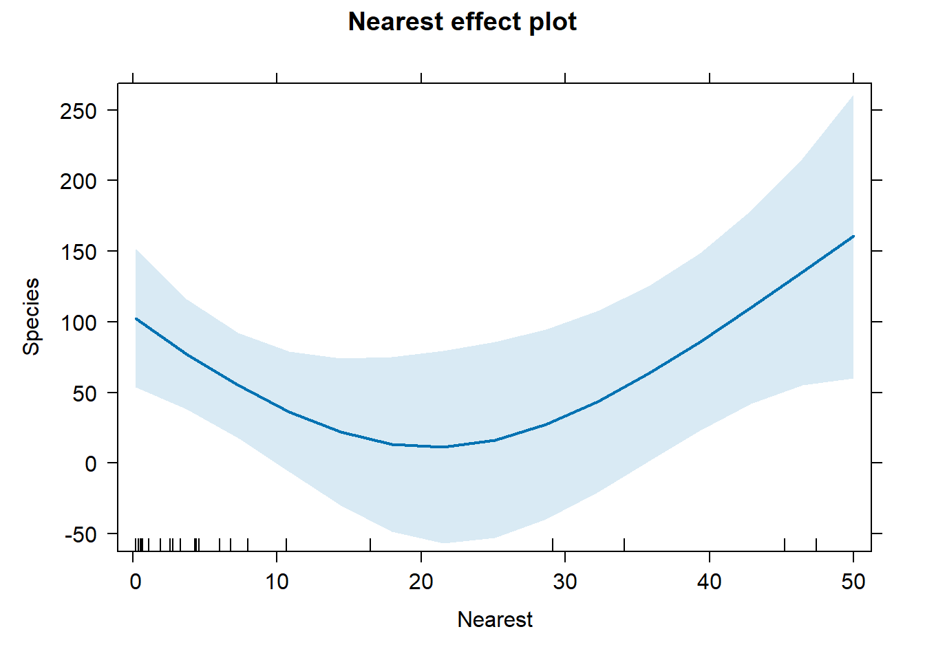
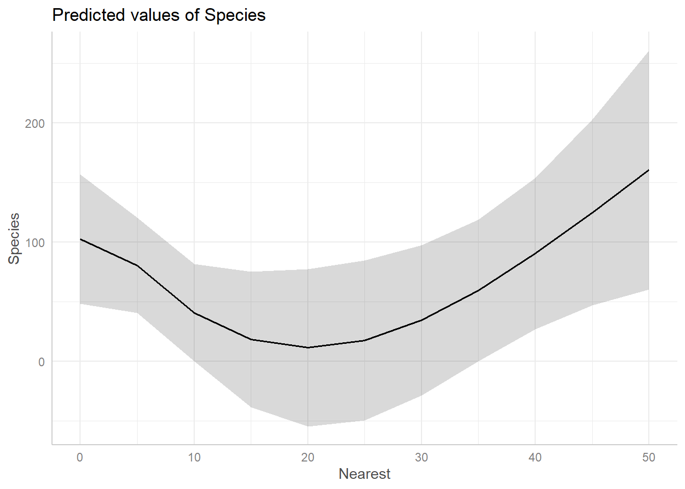
Since interpreting non-linear effect coefficients is all but impossible, we turn to visualization. When fitting a non-linear model with lm(), the {effects} and {ggeffects} packages are fantastic for creating effect plots.
In both cases we see the effect of Nearest is negative for values 0 - 20, but then seems to increase for values above 20.
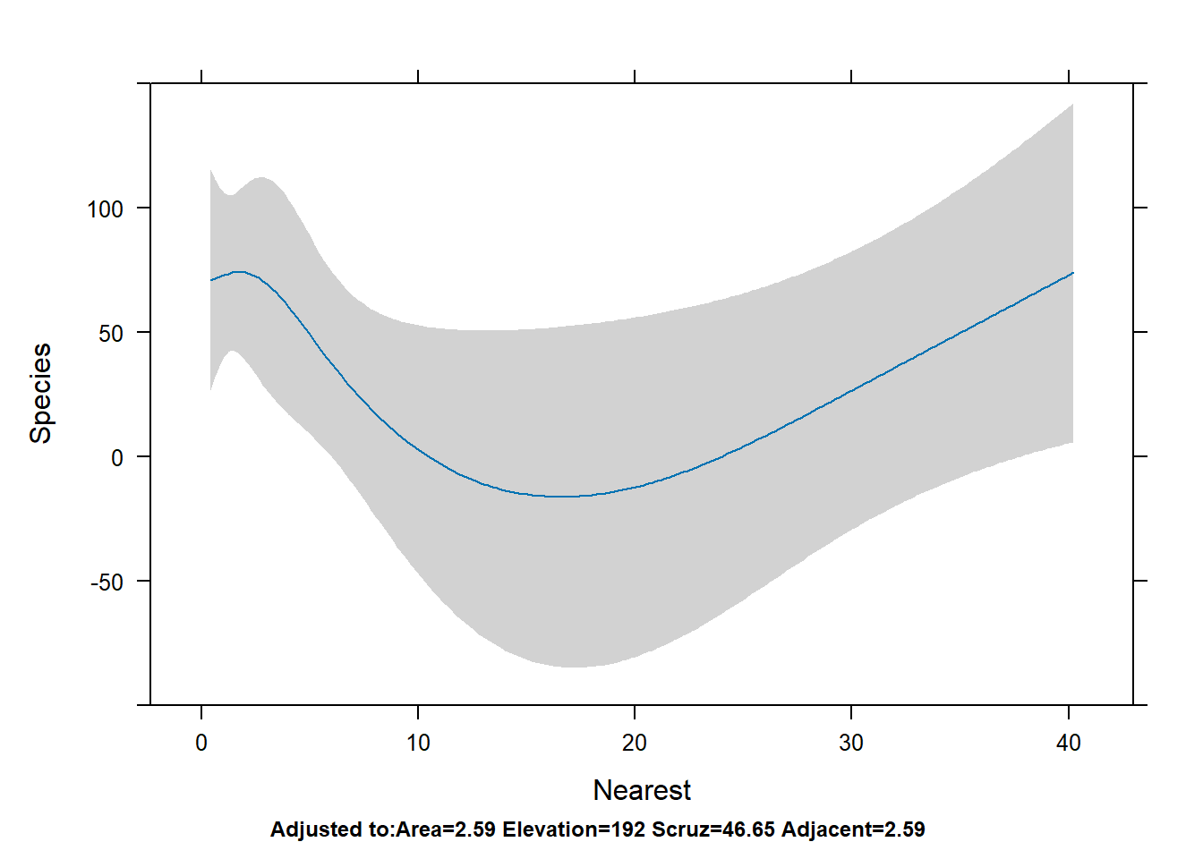
To get a similar plot for an {rms} model, we can use the Predict() function (note the capital “P”; this is an {rms} function) and then pipe into plot(). You can also pipe into ggplot() and plotp() to get ggplot2 and plotly plots, respectively.
Predict(mr2, Nearest) |>plot()
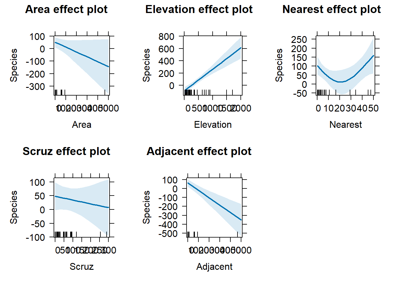
To get all effect plots in one go, we can use the allEffects() function with the lm() model.
allEffects(m2) |>plot()
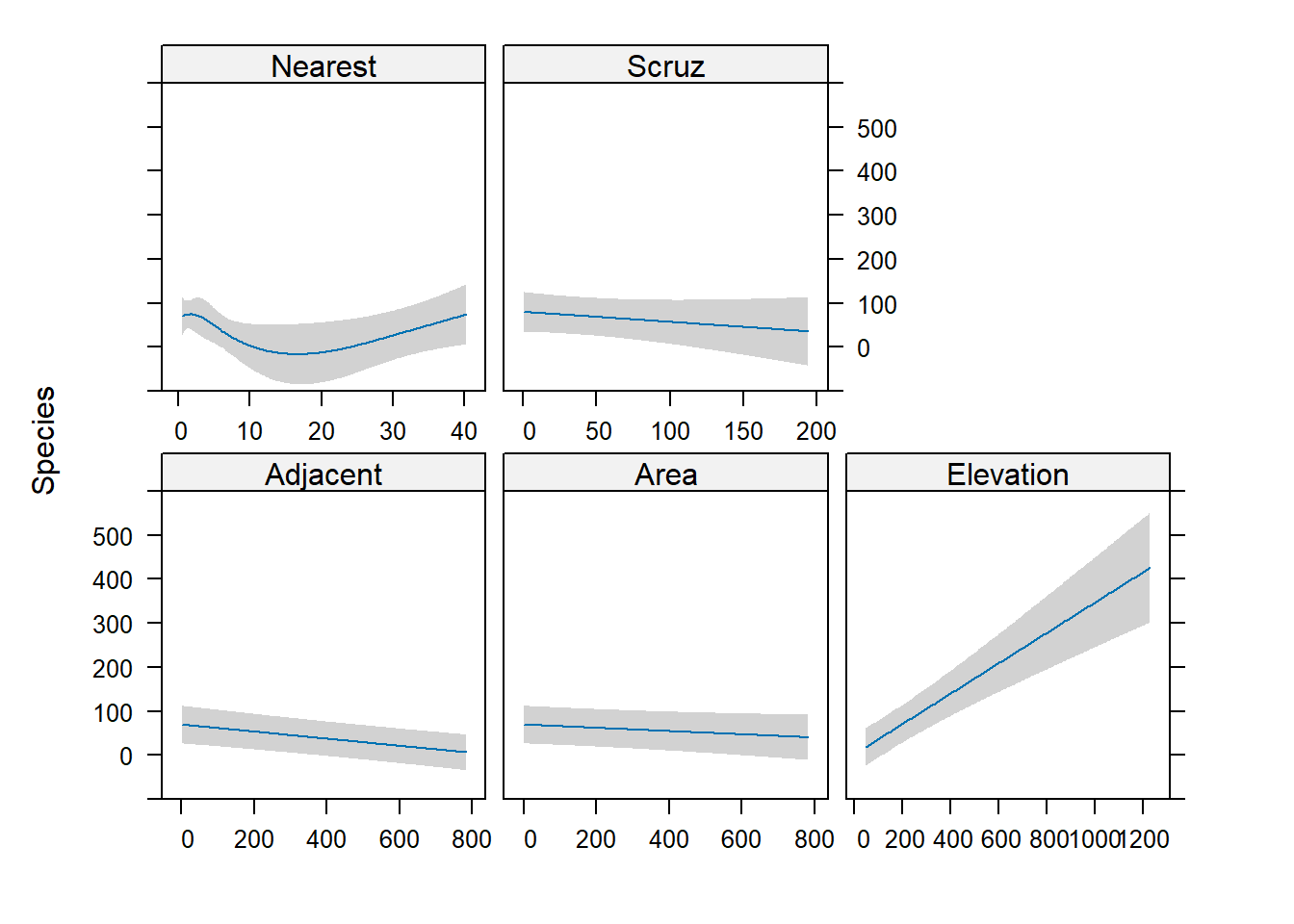
To do the same with {rms}, we use the Predict() function with no predictors specified. Notice the y-axis has the same limits for all plots.
Predict(mr2) |>plot()
Diagnostics
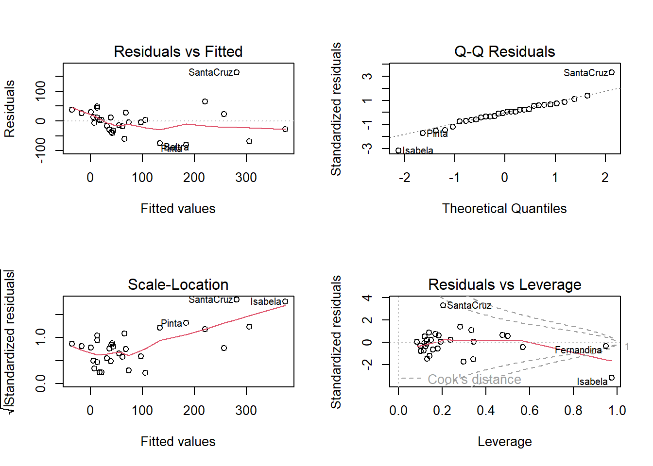
A linear model makes several assumptions, two of which are constant variance of residuals and normality of residuals. The plot() method for lm() objects makes this easy to assess graphically.
op <-par(mfrow =c(2,2))plot(m2)
par(op)
The left two plots assess constant variance using two different types of residuals. The upper right plot assess normality. The bottom right helps identify influential observations. The islands of Isabela and Santa Cruz stand out as either not being well fit by the model or unduly influencing the fit of the model.
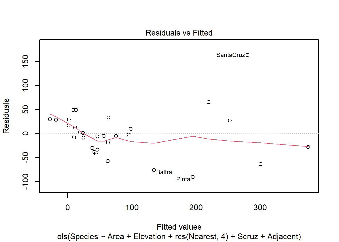
We can use the plot.lm() method on the ols() model, but only the first one (i.e., which = 1).
plot(mr2, which =1)
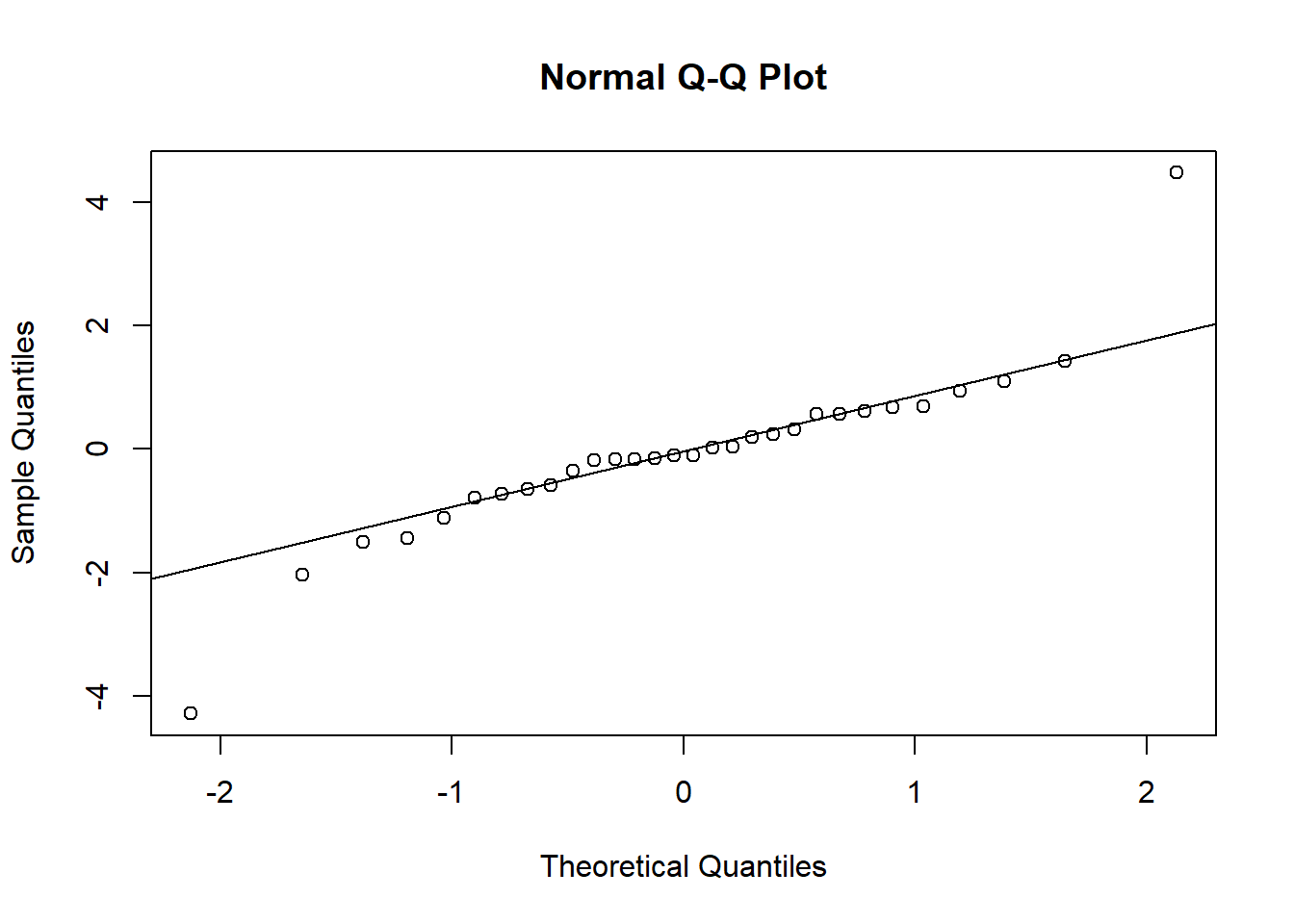
To create a QQ plot to assess normality of residuals we need to extract the residuals using the residuals() function and plot with qqnorm() and qqline()
r <-residuals(mr2, type="student")qqnorm(r)qqline(r)
To check for possible influential observations for an lm() model we can use the base R function influence.measures() and its associated summary() method. See ?influence.measures for a breakdown of what is returned. The columns that begin “dfb” are the DFBETA statistics. DFBETAS indicate the effect that deleting each observation has on the estimates of the regression coefficients. That’s why there’s a DFBETA for every coefficient in the model.
The {rms} package offers the which.influence() and show.influence() tandem to identify observations (via DFBETAS) that effect regression coefficients with their removal. Below we set cutoff = 0.4. An asterisk is placed next to a variable when any of the coefficients associated with that variable change by more than 0.4 standard errors upon removal of the observation. Below we see that removing the Isabela observation changes four of the coefficients. (Also, this is why we set x = TRUE in our call to ols(), so we could use these functions.) The values displayed are the observed values for each observation.
w <-which.influence(mr2, cutoff =0.4)show.influence(w, gala)
Eventually you may want to buy his book, Regression Modeling Strategies. It’s not cheap, but it’s not outrageous either. Considering how much information, advice, code, examples, and references it contains, I think it’s a bargain. It’s a text that will provide many months, if not years, of study.