y <- numeric(100)
y[1] <- rnorm(n = 1, mean = 0, sd = 2)
for(i in 2:100){
  y[i] <- y[i - 1] + rnorm(n = 1, mean = 0, sd = 2)
}
plot(y, type = "o")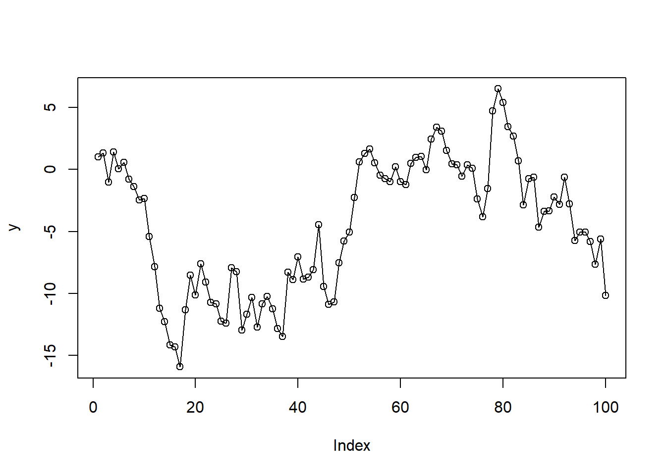
A random walk is a time series constructed as follows
\[Y_t = Y_{t-1} + e_t \]
where the \(e_t\) are independent and identically distributed random variables with mean 0 and a fixed variance, \(\sigma^2\). The initial condition is \(Y_1 = e_1\). Here’s one way to construct a single random walk in R with \(\sigma^2 = 4\) for \(t\) ranging from 1 to 100.
y <- numeric(100)
y[1] <- rnorm(n = 1, mean = 0, sd = 2)
for(i in 2:100){
y[i] <- y[i - 1] + rnorm(n = 1, mean = 0, sd = 2)
}
plot(y, type = "o")
A more efficient way to simulate this in R is using the cumsum() function.
e <- rnorm(n = 100, mean = 0, sd = 2)
y <- cumsum(e)
plot(y, type = "o")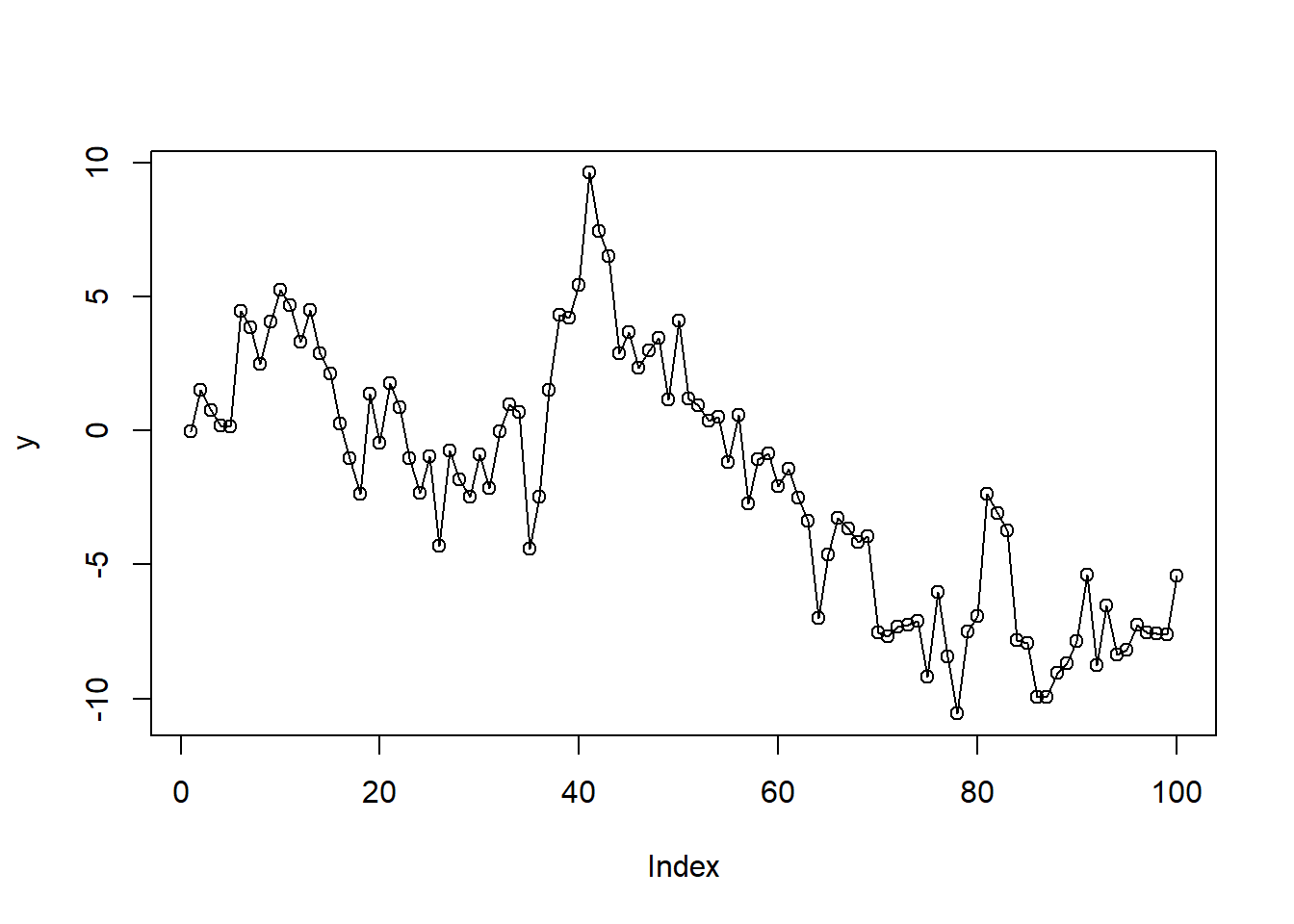
The mean at any time \(t\) in a random walk is 0. To illustrate, let’s generate 100,000 random walks.
rw <- function(t = 100){
  e <- rnorm(n = t, mean = 0, sd = 2)
  y <- cumsum(e)
  y
}

rwalks <- replicate(n = 1e5, rw())
# each column is a random walk
dim(rwalks)
[1] 100 100000Each column is a random walk. To get the mean at time 10, we take the mean of the 10th row. Here I calculate the mean and 95% confidence interval. Notice it’s close to 0.
list(mean = mean(rwalks[10,]), ci = t.test(rwalks[10,])$conf.int)$mean
[1] -0.03555649
$ci
[1] -0.074753142 0.003640166
attr(,"conf.level")
[1] 0.95The mean at time 85 is also about 0.
list(mean = mean(rwalks[85,]), ci = t.test(rwalks[85,])$conf.int)$mean
[1] 0.004338651
$ci
[1] -0.1099330 0.1186103
attr(,"conf.level")
[1] 0.95The variance at time t increases linearly with time:
\[\text{Var}(Y_t) = t\sigma_{t}^2\]
From our random walks above, the variance at time = 10 should be about 10 * 4 = 40.
var(rwalks[10,])[1] 39.99367Likewise, the variance at time = 85 should be about 85 * 4 = 340.
var(rwalks[85,])[1] 339.9151Since each time point is independent of all other time points, the covariance between any two time points, say t and s, such that \(1 \le t \le s\), is also \(t\sigma_{e}^2\).
The covariance between time points 10 and 11 should be about 10 * 4 = 40.
cov(rwalks[10,], rwalks[11,])[1] 39.95689Likewise, the covariance between time points 10 and 85 should also be about 10 * 4 = 40.
cov(rwalks[10,], rwalks[85,])[1] 39.75404The autocorrelation between two time points, t and s, such that \(1 \le t \le s\) is as follows:
\[\rho_{t, s} = \frac{\text{Cov}(Y_t,Y_s)}{\sqrt{\text{Cov}(Y_t,Y_t), \text{Cov}(Y_s,Y_s)}}\]
\[\rho_{t, s} = \frac{t\sigma_{e}^2}{\sqrt{t\sigma_{e}^2 s\sigma_{e}^2}} \]
Which simplifies to:
\[\rho_{t, s} = \frac{t\sigma_{e}^2}{\sqrt{t\sigma_{e}^2 s\sigma_{e}^2}} \frac{\sqrt{t\sigma_{e}^2}}{\sqrt{t\sigma_{e}^2}} = \frac{t\sigma_{e}^2\sqrt{ t\sigma_{e}^2}}{t\sigma_{e}^2\sqrt{s\sigma_{e}^2}} = \sqrt{\frac{t}{s}}\]
Therefore the autocorrelation between time points 10 and 11 should theoretically be \(\sqrt{10/11} \approx 0.953\).
cor(rwalks[10,], rwalks[11,])[1] 0.9532911Likewise, the the autocorrelation between time points 10 and 85 should theoretically be \(\sqrt{10/85} \approx 0.343\).
cor(rwalks[10,], rwalks[85,])[1] 0.3409576The values of Y at neighboring time points are more and more strongly and positively correlated as time goes by.
cor(rwalks[1,], rwalks[2,])[1] 0.7053923cor(rwalks[20,], rwalks[21,])[1] 0.976116cor(rwalks[50,], rwalks[51,])[1] 0.9900396We can visualize this using a simple for loop:
corrs <- numeric(99)
for(i in 1:99){
  corrs[i] <- cor(rwalks[i,], rwalks[i + 1,])
}
plot(corrs, type = "l")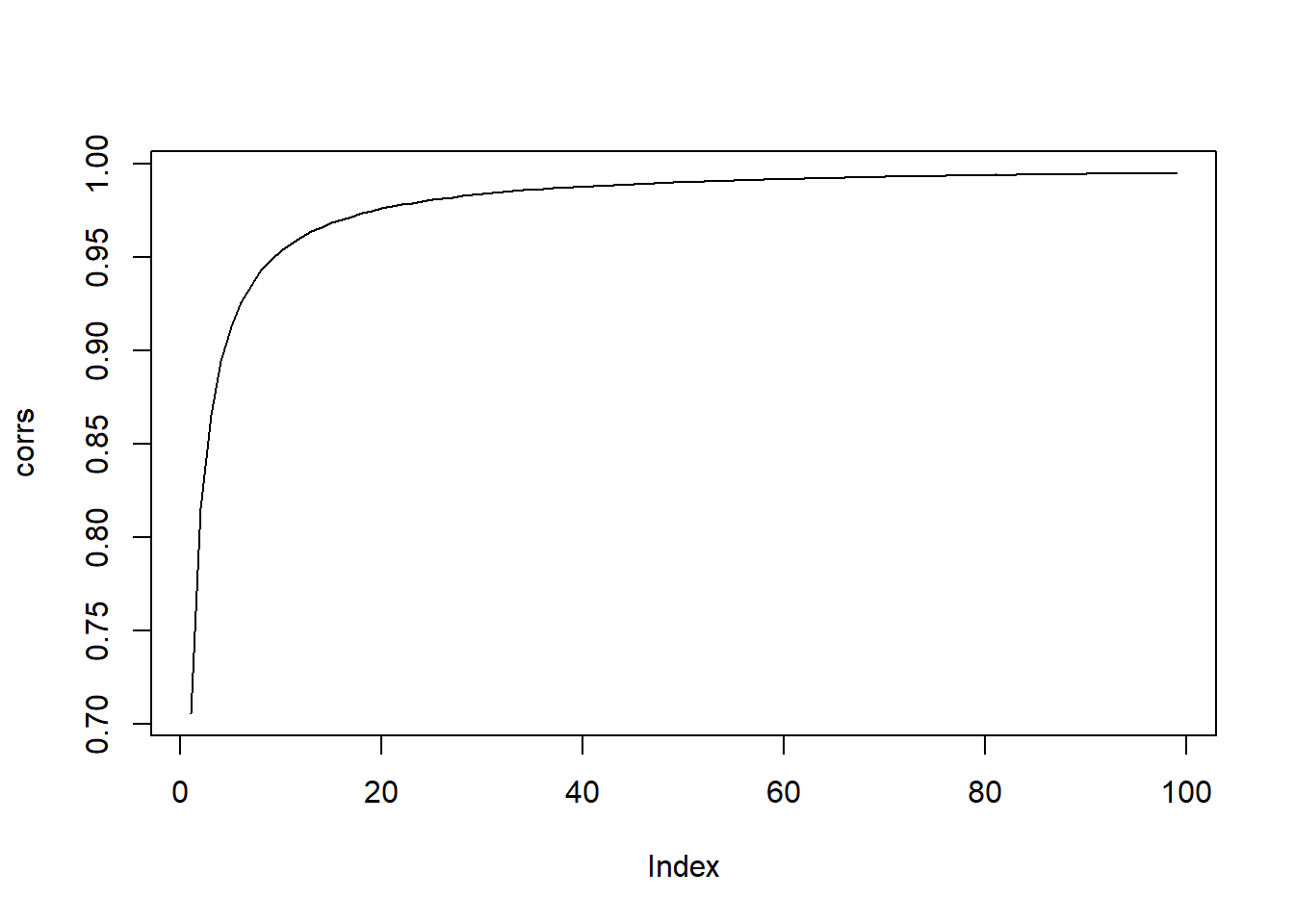
The values of y at distant time points are less and less correlated
cor(rwalks[1,], rwalks[2,])[1] 0.7053923cor(rwalks[1,], rwalks[12,])[1] 0.2857872cor(rwalks[1,], rwalks[30,])[1] 0.1776648Again, pretty easy to visualize:
corrs <- numeric(99)
for(i in 1:99){
  corrs[i] <- cor(rwalks[1,], rwalks[i + 1,])
}
plot(corrs, type = "l")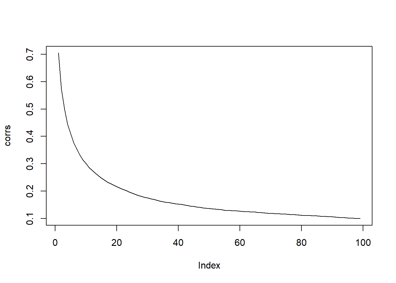
Since variance increases over time and correlation between values nearby in time are close to 1, we should expect long excursions from the mean level of 0. That’s precisely what we see in these nine random walks.
op <- par(mfrow = c(3,3), mar = c(2,2,1,2) + 0.1)
for(i in 1:9) plot(rwalks[,i], type = "l", ylab = "")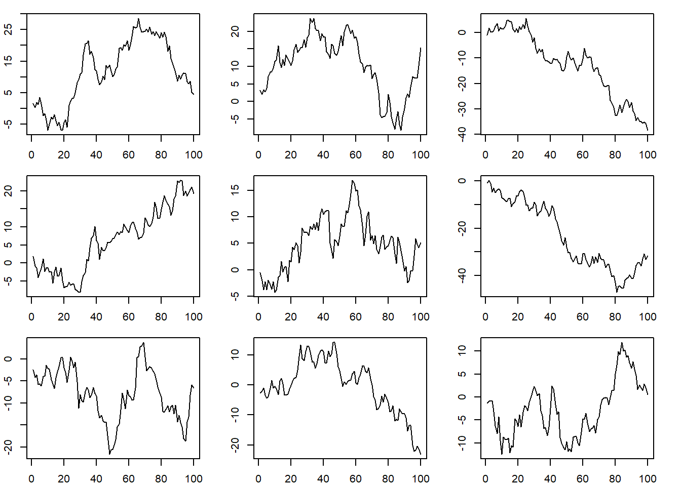
par(op)