set.seed(12)
x <- rpois(n = 3, lambda = 3)
x
[1] 1 5 6This post contains notes on using R’s optim() function. This was originally an informal presentation to colleagues at the University of Virginia in March 2023.
Simulate data from a Poisson distribution.
set.seed(12)
x <- rpois(n = 3, lambda = 3)
x[1] 1 5 6Estimate the mean:
mean(x)[1] 4Given the data, we think the most likely value of lambda is 4. (The true value is 3.) The mean in this case happens to be the maximum likelihood estimator.
The Poisson probability mass function, where \(\lambda\) is the mean:
\[ P(X = x|\lambda) = \frac{e^{-\lambda}\lambda^x}{x!}\] For example, probability of obtaining 5 when \(\lambda = 3\):
\[P(X = 5|\lambda = 3) = \frac{e^{-3}3^5}{5!} \approx 0.101 \]
“By hand” in R:
exp(-3)*(3^5)/factorial(5)[1] 0.1008188Easier to use the dpois() function:
dpois(x = 5, lambda = 3)[1] 0.1008188In the maximum likelihood approach, we find the value of \(\lambda\) that maximizes the product of the probabilities for the data we observed:
\[P(X = 1|\lambda)P(X = 5|\lambda)P(X = 6|\lambda)\]
We could try different values manually:
# max likelihood for lambda = 2
dpois(1, lambda = 2) *
  dpois(5, lambda = 2) *
  dpois(6, lambda = 2)
[1] 0.0001175112Or with less code and R’s vectorization:
# max likelihood for lambda = 2
prod(dpois(c(1, 5, 6), lambda = 2))
[1] 0.0001175112# max likelihood for lambda = 4
prod(dpois(c(1, 5, 6), lambda = 4))[1] 0.0011930884 is more likely than 2 according to these products. The products themselves are not important. We simply want to find the maximum value for a given \(\lambda\).
For computing purposes, it’s easier to take the log of the probability distribution and then sum. (Recall: taking log of products turns into the sum of logs.) The dpois() function includes the log argument to make this easy.
# max log likelihood for lambda = 2
sum(dpois(c(1, 5, 6), lambda = 2, log = TRUE))
[1] -9.048977# max log likelihood for lambda = 4
sum(dpois(c(1, 5, 6), lambda = 4, log = TRUE))[1] -6.731211Again the values are not important, we just want the lambda with the highest log likelihood.
We could try lots of lambdas and find the lambda that returns the highest log likelihood as follows:
x <- seq(1, 10, 0.1) # 1, 1.1, 1.2, ...., 9.8, 9.9, 10
ll <- sapply(X = x,
              FUN = function(x)sum(dpois(c(1, 5, 6),
                                         lambda = x, log = TRUE)))
# which lambda produces max log likelihood?
x[which.max(ll)]
[1] 4Textbooks often visualize this with a plot:
plot(x, ll, type = "l")
abline(v = x[which.max(ll)])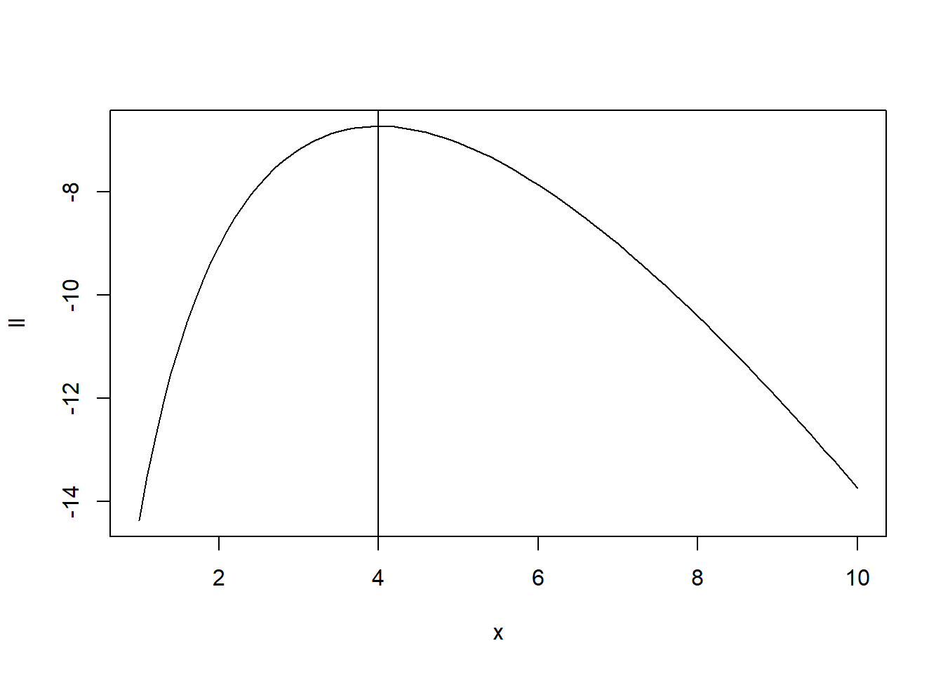
It can be shown using some calculus that the simple mean of the values is the maximum likelihood estimator.
optim()Let’s simulate data from a Poisson distribution where lambda is conditional according to a function of 0.6 + 1.2*x1 + 1.4*x2 - 0.9*x1*x2. We use exp() to ensure the function returns a positive value for lambda, which is required for a Poisson distribution.
n <- 400
set.seed(1)
x1 <- rnorm(n)
x2 <- rnorm(n)
y <- rpois(n = n, lambda = exp(0.6 + 1.2*x1 + 1.4*x2 - 0.9*x1*x2))
head(y)
[1] 4 15 1 9 1 0Imagine we don’t know what process generated this data but we think it came from a Poisson distribution with lambda conditional on the following function: b0 + b1*x1 + b2*x2 + b3*x1*x2 (which is correct). And we wish to use maximum likelihood to estimate the parameters: b0, b1, b2, and b3.
We could again try different values:
# try different b parameters
sum(dpois(y, lambda = exp(0.4 + 1.3*x1 + 1.4*x2 + 0.6*x1*x2), log = TRUE))
[1] -105837.7sum(dpois(y, lambda = exp(0.4 + 1.4*x1 + 1.3*x2 + 0.7*x1*x2), log = TRUE))[1] -152969.1sum(dpois(y, lambda = exp(0.4 + 1.5*x1 + 1.2*x2 + 0.8*x1*x2), log = TRUE))[1] -221947.3We could also turn into a function to make trying values easier.
ll <- function(beta)sum(dpois(x = y, lambda = exp(beta[1] +
                                                    beta[2]*x1 +
                                                    beta[3]*x2 +
                                                    beta[4]*x1*x2),
                               log = TRUE))
ll(beta = c(0.4, 1.3, 1.4, 0.6))
[1] -105837.7ll(beta = c(0.4, 1.4, 1.3, 0.7))[1] -152969.1ll(beta = c(0.4, 1.5, 1.3, 0.8))[1] -317848.3But instead of trying numbers, let’s use an optimization algorithm. The base R optim() provides this service. It offers 6 different optimization algorithms. The default is one called “Nelder-Mead”. See the help page for more details and references.
Now optim() minimizes the objective function so we need to modify our function to return the negative log-likelihood.
# add `-` in front of dpois
ll <- function(beta)sum(-dpois(x = y, lambda = exp(beta[1] +
                                                    beta[2]*x1 +
                                                    beta[3]*x2 +
                                                    beta[4]*x1*x2),
                               log = TRUE))
Now we’re ready to use optim(). The only catch is we need to supply initial values for the function to be optimized. Let’s start with 1 for all parameters.
maxll <- optim(par = c(1, 1, 1, 1), fn = ll)
maxll
$par
[1] 0.6082687 1.1790786 1.3808820 -0.9042680
$value
[1] 698.3295
$counts
function gradient
181 NA
$convergence
[1] 0
$message
NULLWe can extract the parameters as follows:
maxll$par[1] 0.6082687 1.1790786 1.3808820 -0.9042680If we set hessian = TRUE we can get estimated standard errors for the estimated parameters.
maxll <- optim(par = c(1, 1, 1, 1), fn = ll, hessian = TRUE)
maxll$hessian
[,1] [,2] [,3] [,4]
[1,] 2544.174 1789.987 1397.558 -1618.187
[2,] 1789.987 4734.917 -1618.186 -1984.270
[3,] 1397.558 -1618.186 4852.198 2112.786
[4,] -1618.187 -1984.270 2112.786 7794.589Have to “solve”, or take the inverse of, the Hessian matrix to get the variance, and then take square root of the diagonals to get the standard errors.
maxll$hessian |> solve() |> diag() |> sqrt()[1] 0.04213214 0.02524247 0.02792902 0.01594232This is pretty much what we get when we use glm() to estimate the model parameters. It uses an optimization algorithm called “iteratively reweighted least squares (IWLS)”. See this page for more details and R code.
m <- glm(y ~ x1 + x2 + x1:x2, family = poisson)
summary(m)
Call:
glm(formula = y ~ x1 + x2 + x1:x2, family = poisson)

Coefficients:
            Estimate Std. Error z value Pr(>|z|)
(Intercept)  0.60887    0.04212   14.46   <2e-16 ***
x1           1.17901    0.02524   46.72   <2e-16 ***
x2           1.38003    0.02793   49.42   <2e-16 ***
x1:x2       -0.90403    0.01594  -56.70   <2e-16 ***
---
Signif. codes:  0 '***' 0.001 '**' 0.01 '*' 0.05 '.' 0.1 ' ' 1

(Dispersion parameter for poisson family taken to be 1)

    Null deviance: 5096.1  on 399  degrees of freedom
Residual deviance:  409.3  on 396  degrees of freedom
AIC: 1404.7

Number of Fisher Scoring iterations: 5
There is also the mle() function from the {stats4} package. The function it minimizes requires separate arguments. It has a summary method that returns standard errors of the estimated parameters.
library(stats4)

# instead a single vector, specify different arguments
ll2 <- function(b0, b1, b2, b3)sum(-dpois(x = y,
                                          lambda = exp(b0 + b1*x1 +b2*x2 + b3*x1*x2),
                                          log = TRUE))
mle_out <- mle(ll2, start = c(1, 1, 1, 1))
summary(mle_out)
Maximum likelihood estimation
Call:
mle(minuslogl = ll2, start = c(1, 1, 1, 1))
Coefficients:
Estimate Std. Error
[1,] 0.6088984 0.04211905
[2,] 1.1789938 0.02523835
[3,] 1.3800267 0.02792639
[4,] -0.9040193 0.01594304
-2 log L: 1396.657 optim()Insects lay eggs, but not all the eggs survive.
library(ggplot2)
ggplot(d) +
  aes(x = eggs, y = survivors) +
  geom_jitter(width = 0.1, height = 0.1, alpha = 0.5) +
  labs(x = "number of eggs laid", y = "number of survivors") +
  theme_minimal()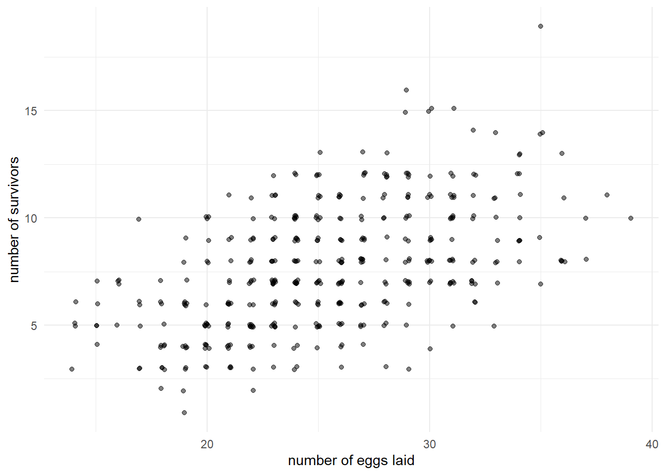
We could model this with a binomial distribution:
\[\text{survivors|eggs laid} \sim \text{binomial}(\text{eggs laid},p)\]
But we could also model number of eggs laid with a Poisson distribution:
\[\text{eggs laid} \sim \text{Poisson}(\lambda)\]
This is an example of a mixture model from Statistical Inference (Casella and Berger). 1
How could we fit such a model and estimate the parameters p and \(\lambda\)? This would be difficult to do using functions such as glm(). However we could use optim() with a custom log likelihood function.
First let’s define our likelihood functions and try different values by hand. We have two probability distributions:
Recall binomial is like a count distribution but capped at size:
# flip 6 fair coins 10 times
rbinom(n = 10, size = 6, prob = 0.5)
[1] 3 3 4 4 2 2 5 4 3 4Sum binomial log likelihood using observed data and different values for p, probability of surviving. We don’t need to do this. Only showing this to motivate use of optim().
# log-likelihood for prob = 0.5
sum(dbinom(x = d$survivors, size = d$eggs, prob = 0.5, log = TRUE))
[1] -1731.607# log-likelihood for prob = 0.4
sum(dbinom(x = d$survivors, size = d$eggs, prob = 0.4, log = TRUE))[1] -1124.161Sum Poisson log likelihood using observed data and different values for lambda.
# log-likelihood for lambda = 2
sum(dpois(x = d$eggs, lambda = 2, log = TRUE))
[1] -17693.09# log-likelihood for lambda = 3
sum(dpois(x = d$eggs, lambda = 3, log = TRUE))[1] -13970.32We can sum these likelihoods and try different values for p and lambda.
# log-likelihood for lambda = 2 and p = 0.5
L1 <- sum(dpois(x = d$eggs, lambda = 2, log = TRUE))
L2 <- sum(dbinom(x = d$survivors, size = d$eggs,
                 prob = 0.5, log = TRUE))
L1 + L2
[1] -19424.7# log-likelihood for lambda = 3 and p = 0.3
L1 <- sum(dpois(x = d$eggs, lambda = 3, log = TRUE))
L2 <- sum(dbinom(x = d$survivors, size = d$eggs,
prob = 0.3, log = TRUE))
L1 + L2[1] -14885.27Now let optim() do the work for us. Remember, we need to make the function negative since optim() minimizes functions.
ll <- function(beta){
  L1 <- sum(dpois(x = d$eggs, lambda = beta[1], log = TRUE))
  L2 <- sum(dbinom(x = d$survivors, size = d$eggs,
                   prob = beta[2], log = TRUE))
  -(L1 + L2)}   # make the function negative

est <- optim(par = c(0.2,0.2), fn = ll, hessian = TRUE)
est$par
[1] 25.4177659 0.3024007Standard errors of the estimated values:
est$hessian |> solve() |> diag() |> sqrt()[1] 0.252069096 0.004555179Note: covariance is 0.
According to our model, eggs are drawn from a Poisson distribution with a mean (lambda) of about 25.4 (se 0.25), and the probability of survival is about 0.3 (se 0.004). Therefore expected number of eggs to survive on average is around 25.4 * 0.3 = 7.622
# P(q > 30)
ppois(q = 30, lambda = est$par[1], lower.tail = FALSE)
[1] 0.156450230 * est$par[2] [1] 9.07202How I simulated the data.
n <- 400
set.seed(2)
eggs <- rpois(n = n, lambda = 25) # number of eggs laid
survivors <- rbinom(n = n, size = eggs, prob = 0.3) # number of survivors
d <- data.frame(eggs, survivors)