The null distribution of deviance

In their book Data Analysis Using Regression and Multilevel/Hierarchical Models, Gelman and Hill state that adding a predictor to a GLM model that doesn’t improve fit will only decrease deviance by about 1. That is also the mean of a chi-square distribution with one degree of freedom, which is the null distribution of deviance between two models with no difference in fit. Let’s simulate this.

Below I simulate two sets of data from a standard normal distribution and generate a binomial outcome using the rbinom() function. Notice I use the plogis() function to make the logit transformation on the linear predictor. Also notice the linear predictor only uses x1. Then I fit two binary logistic regression models: one with just x1 and one with x1 and x2.

set.seed(1)
n <- 500
x1 <- rnorm(n)
x2 <- rnorm(n)
lp <- 0.2 + 0.5*x1
y <- rbinom(n = n, size = 1, prob = plogis(lp))
m1 <- glm(y ~ x1, family = binomial)
m2 <- glm(y ~ x1 + x2, family = binomial)

Since x2 does not improve model fit, we expect the difference in residual deviance between the two models to be about 1.

cbind(m1 = deviance(m1), m2 = deviance(m2))

           m1       m2
[1,] 652.9473 651.8394

The difference in residual deviance can be tested with the anova() function, which you can use when one model is nested within another. In this case m1 is nested within m2 since we can imagine m1 being the same as m2 with a 0 coefficient for the x2 predictor.

anova(m1, m2)

Analysis of Deviance Table

Model 1: y ~ x1
Model 2: y ~ x1 + x2
  Resid. Df Resid. Dev Df Deviance Pr(>Chi)
1       498     652.95                     
2       497     651.84  1   1.1079   0.2925

The deviance listed is 1.1079. The null distribution for deviance when two models are no different and only differ by one coefficient is a chi-square distribution with 1 degree of freedom. Based on the small deviance and large p-value, we fail to reject the null hypothesis of no difference in the fit of the models.

Let’s re-run the simulation above 1000 times and look at the distribution of deviances. The replicate() function makes quick work of this. Notice I save the result of the call to anova() to extract the deviance, which is in the second position of the “Deviance” element.

rout <- replicate(n = 1000, expr = {
  n <- 500
  x1 <- rnorm(n)
  x2 <- rnorm(n)
  lp <- 0.2 + 0.5*x1
  y <- rbinom(n = n, size = 1, prob = plogis(lp))
  m1 <- glm(y ~ x1, family = binomial)
  m2 <- glm(y ~ x1 + x2, family = binomial)
  out <- anova(m1, m2)
  out$Deviance[2]})

As expected, the mean of the deviances is about one.

mean(rout)

[1] 1.023699

Now plot a histogram of the deviances and overlay a chi-square distribution with one degree of freedom. (I used trial-and-error to determine the value of n, which is the number of values used to evaluate the chi-square function.) The deviances are indeed well-modeled with a chi-square distribution.

hist(rout, freq = F, breaks = 50, 
     main = "Distribution of binomial deviances")
curve(expr = dchisq(x, df = 1), from = 0, to = 20, 
      add = TRUE, col = "red", n = 401, lwd = 2)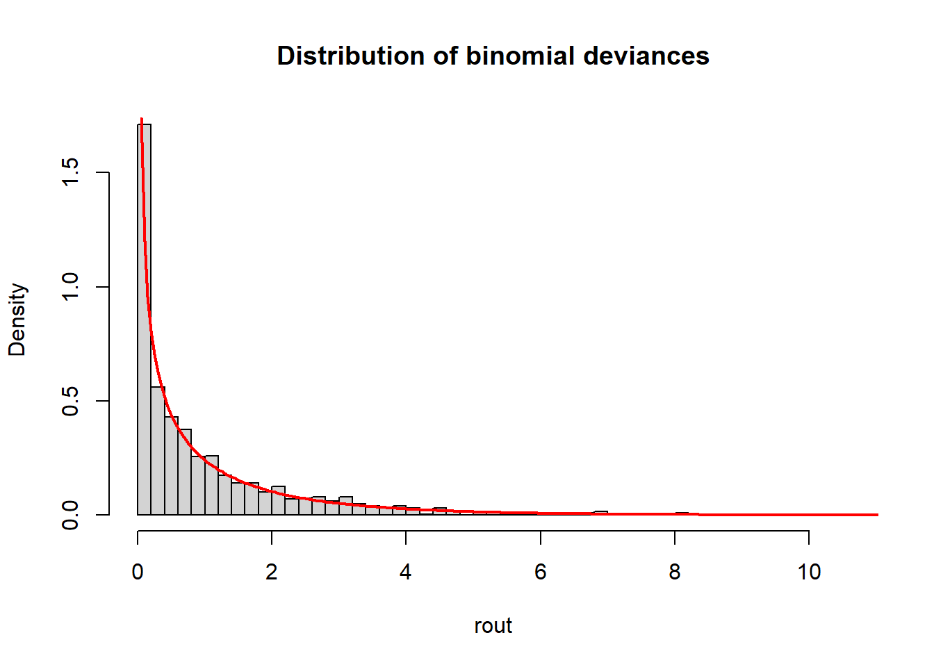

If you prefer a ggplot version, we can do the following. (Again, I had to use trial and error to get the xlim bounds just right.)

library(ggplot2)
d <- data.frame(dev = rout)
ggplot(d) +
  aes(x = dev) +
  geom_density() +
  geom_function(fun = dchisq, args = list(df = 1), color = "red", 
                xlim = c(0.2, 20))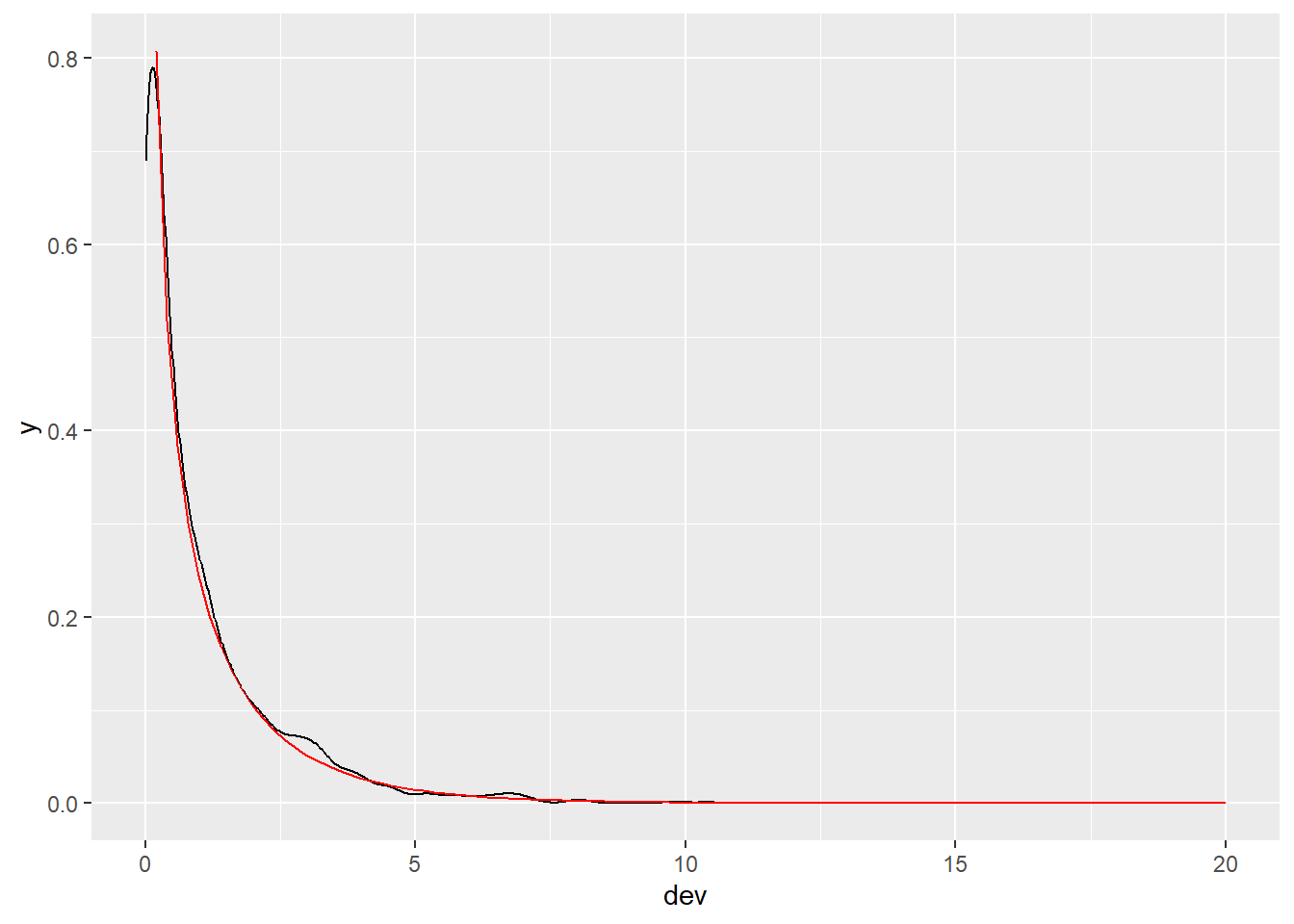

We can also demonstrate this using poisson models.

rout2 <- replicate(n = 1000, expr = {
  n <- 500
  x1 <- rnorm(n)
  x2 <- rnorm(n)
  lp <- 0.2 + 0.5*x1
  y <- rpois(n = n, lambda = exp(lp))
  m1 <- glm(y ~ x1, family = poisson)
  m2 <- glm(y ~ x1 + x2, family = poisson)
  out <- anova(m1, m2)
  out$Deviance[2]})

mean(rout2)

[1] 0.9488272

hist(rout2, freq = F, breaks = 50, 
     main = "Distribution of poisson deviances")
curve(expr = dchisq(x, df = 1), from = 0, to = 20, add = TRUE, col = "red", n = 401, lwd = 2)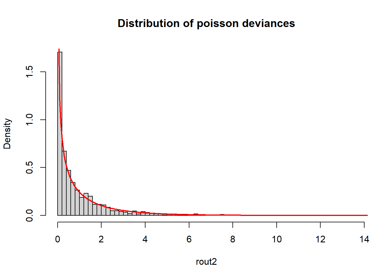

To learn how model residual deviance is calculated, see my UVA Library StatLab article.